This exposition sets out the gain/loss analysis for employee benefit plans as implemented in ProVal. A Glossary of Notation at the end of this exposition defines the variables and terms used.
The gain / loss period may span one year or multiple years. The notation below is written for a one year period. For multiple year periods, the time 1 values (e.g., ![]() ,
,![]() ) should be interpreted as end-of-period values (e.g., for an n year period,
) should be interpreted as end-of-period values (e.g., for an n year period, ![]() ,
,![]() ) and values spanning the one year period of a one year gain /loss analysis (e.g., NC, EB, i) should be interpreted as applying to the entire period (n years for an n year gain / loss analysis).
) and values spanning the one year period of a one year gain /loss analysis (e.g., NC, EB, i) should be interpreted as applying to the entire period (n years for an n year gain / loss analysis).
Overview
The potential sources of gain and loss considered are:
-
Data corrections
-
Active decrements
-
Inactive mortality
-
Salary growth
-
Regulatory increases: U.S. maximum benefit, maximum compensation, social security National Average Wage (NAW) and social security CPI increases; Canadian ITA maximum pension and yearly maximum pensionable earnings (YMPE); German Average Income (West or East), German Current Pension Value (West or East) and German Healthcare BBG; U.K. CPI, RPI, Section 148 Orders and Lower Earnings Limit
-
Database fields for continuing actives
-
New entrants
-
Benefit payments
-
ProVal system changes
-
Non-liability gains or losses (e.g., investment income and expenses)
-
Implicit assumption changes
-
Interest rate changes
The method used is mathematically precise, that is, a source other than one listed above (e.g., a mistake in coding the Valuation(s), service accrual other than expected, COLA other than expected, etc.) will be categorized as "unreconciled".
The total gain, regardless of actuarial cost method, can be expressed as
![]()
where ![]() represents the (experience) gain on assumptions that drive the liabilities,
represents the (experience) gain on assumptions that drive the liabilities,
![]() represents the gain on expenses, and
represents the gain on expenses, and
![]() represents the gain on investment income.
represents the gain on investment income.
The evaluation of![]() and
and![]() is a trivial exercise and is independent of cost method:
is a trivial exercise and is independent of cost method:

A more significant task is the allocation of![]() among the various sources. Intuitively,
among the various sources. Intuitively, ![]() represents the gain in the estimate of the end-of-period liability for benefits to be paid during and after the period of analysis. We can write
represents the gain in the estimate of the end-of-period liability for benefits to be paid during and after the period of analysis. We can write![]() as the difference between the beginning-of-period estimate for this liability (call it
as the difference between the beginning-of-period estimate for this liability (call it![]() ) and the end-of-period estimate (call it
) and the end-of-period estimate (call it![]() , where k is the number of sources of gains and losses to be analyzed). We need to split
, where k is the number of sources of gains and losses to be analyzed). We need to split![]() into pieces. To do that, we’ll construct a sequence
into pieces. To do that, we’ll construct a sequence ![]() for i=0…k. We already know what
for i=0…k. We already know what![]() and
and![]() represent. The intermediate
represent. The intermediate ![]() are also estimates for the same liability. They are calculated by successively replacing assumptions with experience. Thus the difference between values of sequential elements,
are also estimates for the same liability. They are calculated by successively replacing assumptions with experience. Thus the difference between values of sequential elements, ![]() and
and ![]() , is the gain or loss due to those assumptions inherent in
, is the gain or loss due to those assumptions inherent in![]() that we replaced with experience when calculating
that we replaced with experience when calculating![]() . The expression for
. The expression for ![]() becomes a telescoping series:
becomes a telescoping series:

where![]() is the gain due to source i. Each
is the gain due to source i. Each![]() in the sequence is itself the sum of individual values
in the sequence is itself the sum of individual values![]() calculated for each participant j.
calculated for each participant j.
General form of![]() for the immediate gain recognition cost methods:
for the immediate gain recognition cost methods:
Appendix A derives the following result for immediate gain recognition cost methods:
![]()
![]()
Recall that each![]() represents an estimate of the end-of-period liability for benefits to be paid during and after the period. It’s clear that
represents an estimate of the end-of-period liability for benefits to be paid during and after the period. It’s clear that ![]() meets this definition. A little rearrangement of terms will demonstrate that
meets this definition. A little rearrangement of terms will demonstrate that![]() does too:
does too:
![]()
Elements of the sequence based on beginning-of-period Valuation(s) will be in the form of![]() ; those based on end-of-period Valuation(s) will be in the form of
; those based on end-of-period Valuation(s) will be in the form of![]() . If the gain / loss period spans more than one year, all elements of the sequence will span the entire period and, instead of a beginning-of-period valuation, a core projection is run through the end of the period, with a baseline valuation date at time 0.
. If the gain / loss period spans more than one year, all elements of the sequence will span the entire period and, instead of a beginning-of-period valuation, a core projection is run through the end of the period, with a baseline valuation date at time 0.
General form of![]() for the spread gain recognition cost methods:
for the spread gain recognition cost methods:
Appendix B derives the following result for spread gain recognition cost methods:

Although it may not be quite as obvious, these expressions also conform to our intuitive definition: estimates of the end-of-period liability for benefits to be paid during and after the period. The first three terms of each expression represent the present value of benefits that are not to be paid by future normal costs – that is, they represent the liability we have already accrued. Using![]() instead of
instead of![]() in our expression for
in our expression for![]() essentially "turns off" the spreading of the gain or loss and causes the gain or loss to become a part of this liability, instead of part of the present value of future normal costs. As for the immediate gain recognition methods, normal cost (both employee and employer) is added to
essentially "turns off" the spreading of the gain or loss and causes the gain or loss to become a part of this liability, instead of part of the present value of future normal costs. As for the immediate gain recognition methods, normal cost (both employee and employer) is added to![]() and benefits are added to
and benefits are added to![]() .
.
Constructing the sequence {![]() }
}
This section discusses the liability sequence by way of an example with 20 elements, reflecting analysis by source of U.S. regulatory items. In practice, the sequence may have any number of elements, k.
-
Beginning-of-period Valuation(s):

The first element of the sequence,
, will be calculated from the previously run (and saved) beginning-of-period Valuation(s). This element is not available if the gain / loss period is longer than one year.
-
Beginning-of-period Valuation(s), re-executed:

The next element,
, is computed by re-executing the beginning-of-period Valuation(s). If the gain / loss period is longer than one year, a core projection is run (instead of a valuation) to project the liabilities to the end of the period.
-
Data corrections:

If a database containing corrected beginning-of-period data is supplied, ProVal uses that database to calculate the next element of the sequence. The corrected data will be used in combination with the same Census Specifications, Valuation Assumptions and Plan Definition that were used to calculate
.
-
Active decrements:
 ,
,  ,
,  ,
, 
The next four elements successively replace the time 0 (assumed) probabilities of retirement, termination, death and disability with experience, so that
reflects the actual end-of-period status of each participant who was active at time 0. We don’t actually run any of these valuations – we simulate them, using individual results from our last time 0 runs (i.e., the runs used to calculate
). See Appendix C for a discussion of the calculations involved.
-
Inactive mortality:
 ,
,  ,
,  ,
, 
The next four elements successively replace the time 0 (assumed) probabilities of mortality for members (retired, vested terminated and disabled) and beneficiaries (including survivors) with experience, so that
reflects the actual end-of-period status of each member and beneficiary who was an inactive participant at time 0. Just as for active decrements, we don’t actually run any of these valuations – we simulate them, using individual results from our last time 0 runs (i.e., the runs used to calculate
). See Appendix D for a discussion of the calculations involved.
-
Salary growth, regulatory increases and database fields:
 ,
, ,
, , …,
, …, 
The next several elements replace the expected values for salaries, regulatory data and database fields with experience for each continuing active participant. These items are divided into one or more groups, or sources, in the order indicated by the user. Note that the order will affect the allocation of gains and losses.
Eachis computed by running the end-of-period valuation(s) – note that the computation must be at the end of the period because we’ve already replaced decrement assumptions with the end-of-period status of “active” in our analysis of active decrements above.
Before doing these runs,is recomputed, using time 0 salary and regulatory data but the end-of-period database (with expected values for selected continuing active sources in lieu of actual values), and end of period Valuation Assumptions and Plan Definition. Any difference between recomputed
and
from the end-of-period valuations is categorized as unreconciled. For possible sources of unreconciled amounts, see the discussion in the article on Gain/Loss Analysis Output.
-
New entrants:

The next element,
, adds to
the amount of liability attributable to new entrants.
-
Benefit payments:

The next element,
, adds to
the difference between expected and actual benefit payments for the period (with interest to the end of the period).
-
End-of-period Valuation(s), re-executed using assumptions consistent with the beginning of period:

The next element,
, is computed by re-executing the end-of-period Valuation(s) using assumptions, for dynamic mortality and for interest rates that are variable by duration from the valuation date, that are consistent with the beginning of period valuation. This means using (1) the mortality table assumed in the beginning-of-period Valuation(s) (based on the beginning-of-period valuation date) and (2) the end-of-period spot rate curve implied by the beginning-of-period assumed interest rates (see the Technical Reference article entitled “Gain and loss analysis: U.S. PPA Target Liabilities ” for a detailed discussion in the context of the PPA interest rate structure).
-
Implicit assumption changes:

 ,
,  ,
, 
The next three elements determine the implicit assumption change due to dynamic mortality, interest rates that vary by duration from the valuation date, and other assumptions where a roll-forward of beginning of period liability does not perfectly match end of period liability, respectively.
The implicit assumption change due to dynamic mortality,
, is computed by re-executing the end-of-period Valuation(s) using interest rate assumptions that are consistent with the beginning of period valuation and the dynamic mortality assumption, which is as of the end of period valuation date.
The implicit assumption change due to interest rates that vary by duration from the valuation date,
, is computed by re-executing the end-of-period Valuation(s) using end of period dynamic mortality and an end of period interest rate assumption cosmetically identical to the beginning of period interest rate assumption. In other words, if the beginning of period assumption uses interest rates of X, Y, and Z, which vary by duration x, y, and z from the beginning of period valuation date, then this end of period valuation will use interest rates of X, Y, Z, varying by duration x, y, and z from the end of period valuation date.
The implicit assumption change due to other assumptions where a roll forward of beginning of period liability does not perfectly match end of period liability,
, is computed by capturing a comparison of the beginning of period liability roll-forward to the end of period baseline (disregarding all other gain and loss elements). This calculation is done immediately following data corrections and is added in at this stage.
-
Interest rate changes – End-of-period Valuation(s), re-executed:

The next element of the sequence,
, is computed by re-executing the end-of-period Valuation(s) with end-of-period assumptions. This valuation will be executed only if end of period valuation interest assumptions are distinct from beginning of period valuation interest assumptions. (For example, if, as is typical, U.S. qualified single-employer plan segment interest rates in the end of year valuation are different from the segment rates in the beginning of year valuation, then these assumptions are distinct.) Else,
and
will yield identical results.
-
End-of-period Valuation(s):

The last element of the sequence,
, will be calculated from the previously run (and saved) end-of-period Valuation(s).
Taking the first difference of the sequence {![]() }, we obtain the following results.
}, we obtain the following results.
| Gain | Source |
| System changes #1 – not available if the valuation period spans more than one year | |
| Data corrections | |
| Active decrement – retirement | |
| Active decrement – termination | |
| Active decrement – death | |
| Active decrement – disability | |
| Inactive mortality – retired members | |
| Inactive mortality – vested terminated | |
| Inactive mortality – disabled members | |
| Inactive mortality – survivor beneficiaries | |
| Salary growth, regulatory increases, database fields (source 1) | |
| Salary growth, regulatory increases, database fields (source 2) | |
| Salary growth, regulatory increases, database fields (source 3) | |
| … | … |
| Salary growth, regulatory increases, database fields (source n) | |
| New entrants | |
| Benefit payments | |
| Unreconciled | |
| Implicit assumption change due to mortality | |
| Implicit assumption change due to interest rates | |
| Implicit assumption change due to other | |
| Interest rate change | |
| System changes #2 |
For simplicity’s sake, the total system change can be represented as x0 – x1+ x10+(n+7) – x10+(n+8).
The unreconciled amounts, x10+(n+2) – x10+(n+3), deserve further explanation and are discussed in the article Gain/Loss Analysis Output.
Appendix A
General form of![]() for immediate gain recognition methods
for immediate gain recognition methods
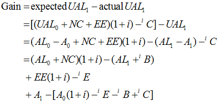
For these cost methods, the gain is the difference between expected and actual unfunded liabilities:
Clearly defining the elements

will provide the desired result
![]()
It may be more instructive to think of GL as

Appendix B
General form of![]() for spread gain recognition methods
for spread gain recognition methods
The gain or loss under these methods shows up in the present value of employer-paid future normal costs:

![]() is the dollar amount of the gain. As required, this equation yields a zero result if all assumptions are met exactly, because, in that case,
is the dollar amount of the gain. As required, this equation yields a zero result if all assumptions are met exactly, because, in that case, ![]() .
. ![]() is also a number worth presenting. It represents the change in normal cost rate from gains during the period, rather than the dollar amount of those gains.
is also a number worth presenting. It represents the change in normal cost rate from gains during the period, rather than the dollar amount of those gains.
The dollar amount of the gain can be decomposed as follows:
![]()
where, for a U.S. qualified plan,

Substituting and rearranging, we have
 So, once again, we can achieve the desired result
![]()
by making the definitions

The derivation shown here is based on the (U. S. qualified plan) balance equation, which may fail when a plan has hit the full funding limitation and has a funding standard account credit balance. But if we allow the value of the UAL to go negative, the math holds together even in that situation.
Appendix C
![]() for Incidence of Decrement
for Incidence of Decrement
The gain due to incidence of a decrement is calculated, like any other gain, as the difference between sequential elements. The relevant values are unlike the others in our sequence because they are algebraically derived, rather than calculated directly from valuations. There are two basic reasons for this difference:
-
We will construct a sequence of four elements that successively replace a decrement assumption with actual experience. All of the benefits and liabilities that would arise from the decrements will be the same as in the previous element. If we have saved this information for each individual, then we can avoid doing four valuations. The time saved will be considerable.
-
The intermediate values in this subsequence will use inconsistent assumptions. For example, one of them may value an individual as having terminated during the year but also with a nonzero probability of having died. Clearly, this is an inconsistent assumption set with which to perform a valuation.
So what are the relevant expressions? Once again, we will consider immediate gain and spread gain cost methods separately. Keep in mind that these calculations will be based on time 0 valuations and will reflect, in part or in whole, actual end-of-period status.
Immediate gain recognition method![]() :
:
Let![]() be an element based on the time 0 Valuation(s) with the actuarial assumptions used for all decrements. If we define the following terms,
be an element based on the time 0 Valuation(s) with the actuarial assumptions used for all decrements. If we define the following terms,
![]() Accrued liability at end-of-period, if active participant continues in active status
Accrued liability at end-of-period, if active participant continues in active status
![]() Accrued liability at end-of-period, if active participant decrements from cause k during the last year of the period. The decrement occurs either at the beginning or the middle of the year, depending on the decrement timing selected in Valuation Assumptions.
Accrued liability at end-of-period, if active participant decrements from cause k during the last year of the period. The decrement occurs either at the beginning or the middle of the year, depending on the decrement timing selected in Valuation Assumptions.
![]() Beginning-of-period value of expected benefits to be paid during the period, if active participant decrements from cause k during the last year of the period. The decrement occurs either at the beginning or the middle of the year, depending on the decrement timing selected in Valuation Assumptions.
Beginning-of-period value of expected benefits to be paid during the period, if active participant decrements from cause k during the last year of the period. The decrement occurs either at the beginning or the middle of the year, depending on the decrement timing selected in Valuation Assumptions.
We can express![]() in the following manner:
in the following manner:
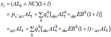
where k ranges over all decrements.
Now suppose xi+1 substitutes withdrawal actual experience for expected. It can be written as

More generally, let J be a set of decrements for which we want to use actual rather than assumed experience. The appropriate statement is

This statement is consistent with our previous definitions. When J=Æ,![]() reduces to the original expression. When
reduces to the original expression. When![]() ,
,

which is the desired result.
This means that we don’t have to do any valuations to calculate our gain from incidence of decrement. We do, however, need to have written out some information from our time 0 valuation. We need ![]() and
and![]() , and we need
, and we need ![]() ,
, ![]() and
and ![]() for each decrement k (term cost can be substituted for
for each decrement k (term cost can be substituted for ![]() and
and ![]() ). Once we have these values, we can calculate the last item we need:
). Once we have these values, we can calculate the last item we need:

Spread gain recognition method![]() :
:
This discussion follows much the same pattern as for the immediate gain recognition method. We can write![]() as
as

If we wish to replace assumptions with experience for a set of decrements J, we can calculate

We must write several items from our time 0 Valuation(s): ![]() ,
, ![]() ,
, ![]() ,
, ![]() , and
, and ![]() , as well as
, as well as ![]() ,
, ![]() , and
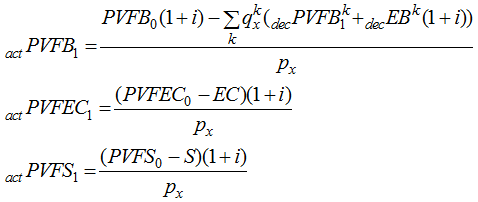
, and ![]() , for each decrement k. The remaining items can be calculated as follows:
, for each decrement k. The remaining items can be calculated as follows:
Adjustments to formulas above to reflect in-service benefits:
When in-service benefits are valued, we must additionally take into consideration the active in-service benefits paid during the period, along with, potentially, a liability due as a result of in-service benefits which have been defined as annuities (rare). These formulas are discussed below.
In-service benefits are most commonly defined as a lump sum due each year in which a participant remains active. Let’s start by looking at this case for a 1-year gain/(loss) analysis:
We previously defined this formula for ![]() which assumed zero benefits paid while in-service:
which assumed zero benefits paid while in-service:

![]()
To reflect in-service benefits in this formula, we must add a term for in-service benefits in each active liability term. Note that in-service benefits are paid before active decrements apply, therefore in a 1-year gain/(loss), both actAL1 and decAL1 must include this term.
Let ![]() be the in-service benefit payments due at the beginning of period valuation date.
be the in-service benefit payments due at the beginning of period valuation date.
The formula for ![]() becomes:
becomes:
![]()
![]()
![]()
which simplifies to:

![]()
Although uncommon, it is possible to define an in-service benefit as an annuity. This would mean each year’s benefit due for in-service would be paid over time, even if the participant terminated in a subsequent year. This formula would be very similar to the one developed above, except that we now must include a term for the liability due as a result of in-service benefits being paid. Similar to the in-service benefit itself, the same amount must be added to both actAL1 and decAL1 and, as a result, will cancel out within the summation.
Let ![]() be the end of period present value of in-service benefit (at time 1), representing benefits payable in the future, but initiated by being active at time 0. Then the formula for
be the end of period present value of in-service benefit (at time 1), representing benefits payable in the future, but initiated by being active at time 0. Then the formula for ![]() becomes:
becomes:

![]()
The comments above apply not only to annuities, but to any payment form that included payments beyond the end of the gain/loss measurement period (e.g. lump sums with deferral or installments). In addition, keep in mind that if the payments are dependent on survival of the member or their spouse, ProVal applies retiree mortality in determining the payment form value. This can result in an unreconciled gain or loss for the following reasons:
-
Experience survival differing from assumed retiree mortality
-
Experience decrement to a status other than active or retired, if the mortality for that status differs from retiree mortality
Finally, we can expand the formula above to consider an n-year (gain)/loss. The n-year gain/(loss) has an additional level of complexity because expected decrements occur in each year of the n-year period, so that, unlike the 1-year gain/(loss), the expected in-service benefit payments are not the same for actAL1 and decAL1.
Let:
![]() be the in-service benefit payments payable over n-years at the beginning of period to the portion of each participant remaining in service.
be the in-service benefit payments payable over n-years at the beginning of period to the portion of each participant remaining in service.
![]() be the end of period present value of in-service benefit (at time n), representing benefits payable in the future to the portion of each participant remaining in service.
be the end of period present value of in-service benefit (at time n), representing benefits payable in the future to the portion of each participant remaining in service.
![]() be the expected in-service benefit payments payable over n-years for the portion of each participant expected to decrement.
be the expected in-service benefit payments payable over n-years for the portion of each participant expected to decrement.
![]() be the end of period present value of in-service benefit (at time n), representing benefits payable in the future to the portion of each participant expected to decrement.
be the end of period present value of in-service benefit (at time n), representing benefits payable in the future to the portion of each participant expected to decrement.
Note that, while expected decrements may occur during each year of the gain/(loss), actual known decrements are assumed to have occurred at time n-1. Therefore the terms in the second summation only will cancel out, yielding:
![]()
![]()
![]()
For spread gain methods, the necessary formula adjustments to reflect in-service benefits are the same as for immediate gain methods, where the expected benefits and corresponding liabilities for in-service benefits are added to each PVFB term. For example, for an n-year gain/(loss) the formula becomes:
![]()

![]()
Appendix D
![]() for Inactive Mortality
for Inactive Mortality
The ![]() calculated for inactive participants is independent of cost method:
calculated for inactive participants is independent of cost method:

Breaking ![]()
![]() into amounts dependent upon survival, we can write an equivalent expression for
into amounts dependent upon survival, we can write an equivalent expression for ![]() :
:
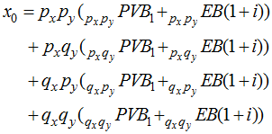
Replacing the primary annuitant’s mortality assumption with experience, we arrive at the next element of the sequence:
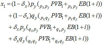
Replacing the mortality assumptions for both annuitants with experience, we arrive at the next element of the sequence:
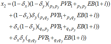
So, for inactive participants, we need to write out qx and qy .for the period. We also need to write out the anticipated PVB at the end of the period and the value of expected benefits to be paid during the period for each of four survival combinations. Deaths are assumed to occur during the last year of the period, with survival up to that point.
Appendix E
Determining ![]() from status transitions
from status transitions
This appendix describes a method of determining experience for active decrements, ![]() , and inactive mortality,
, and inactive mortality, ![]() , by examining the transition from beginning-of-period status to end-of-period status. Each status will take on one of the following values: "active", "retired", "vested", "disabled", "survivor", or "non-participating". The "non-participating" status includes a participant who is omitted from the data, is missing status or is non-participating.
, by examining the transition from beginning-of-period status to end-of-period status. Each status will take on one of the following values: "active", "retired", "vested", "disabled", "survivor", or "non-participating". The "non-participating" status includes a participant who is omitted from the data, is missing status or is non-participating.
Active decrements
For participants who are in "active" status and eligible for inclusion in funding cost at the beginning of the period,
![]() =1 if end-of-period status is "retired" and
=1 if end-of-period status is "retired" and
participant is eligible for retirement at beginning-of-period
![]() =1 if end-of-period status is "vested" and
=1 if end-of-period status is "vested" and
participant is not eligible for retirement at beginning-of-period
![]() =1 if end-of-period status is "survivor"
=1 if end-of-period status is "survivor"
![]() =1 if end-of-period status is "disabled"
=1 if end-of-period status is "disabled"
Inactive mortality
For participants who are in "retired", "vested" or "disabled" status at the beginning of the period,
![]() =1 if end-of-period status is "survivor" or "non-participating"
=1 if end-of-period status is "survivor" or "non-participating"
For participants who are in "survivor" status at the beginning of the period,
![]() =1 if end-of-period status is "non-participating"
=1 if end-of-period status is "non-participating"
For participants with a contingent annuitant (i.e., beneficiary) at the beginning of the period,
![]() =1 if no contingent annuitant exists at end-of-period.
=1 if no contingent annuitant exists at end-of-period.
Exceptions:
1) If ![]() =1 and end-of-period status is "retired", "vested", "disabled" or "survivor" (i.e., inactive), then
=1 and end-of-period status is "retired", "vested", "disabled" or "survivor" (i.e., inactive), then ![]() =0. In other words, if the member died but the participant is still inactive, then the beneficiary must still be alive.
=0. In other words, if the member died but the participant is still inactive, then the beneficiary must still be alive.
2) If beginning-of-year status is "retired", "vested" or "disabled" and end-of-year status is "active" (i.e., rehired), then ![]() =0.
=0.
Glossary of Notation
![]() Decrement flag that is 1 if active participant experienced the decrement k during the period, 0 otherwise
Decrement flag that is 1 if active participant experienced the decrement k during the period, 0 otherwise
![]() Mortality flag that is 1 if inactive participant dies during the period, 0 otherwise
Mortality flag that is 1 if inactive participant dies during the period, 0 otherwise
![]() Accrued liability at time n
Accrued liability at time n
![]() Accrued liability at time 1, if active participant continues in active status
Accrued liability at time 1, if active participant continues in active status
![]() Accrued liability at time 1, if active participant decrements from cause k
Accrued liability at time 1, if active participant decrements from cause k
![]() Valuation assets at time n
Valuation assets at time n
![]() Accumulated reconciliation account at time n (U.S. qualified plans)
Accumulated reconciliation account at time n (U.S. qualified plans)
![]() Credit balance / (accumulated funding deficiency) at time n (U.S. qualified plans)
Credit balance / (accumulated funding deficiency) at time n (U.S. qualified plans)
![]() Beginning-of-period value of expected benefits paid during the period
Beginning-of-period value of expected benefits paid during the period
![]() Beginning-of-period value of expected benefits to be paid during the period, if an active participant decrements from cause k
Beginning-of-period value of expected benefits to be paid during the period, if an active participant decrements from cause k
![]() Beginning-of-period value of employee contributions to be made during the period
Beginning-of-period value of employee contributions to be made during the period
![]() Beginning-of-period value of estimated expenses for the period that are included in funding cost
Beginning-of-period value of estimated expenses for the period that are included in funding cost
![]() Normal cost rate computed in time n valuation
Normal cost rate computed in time n valuation
![]() Total gain or (loss)
Total gain or (loss)
![]() Gain or (loss) from expenses
Gain or (loss) from expenses
![]() Gain or (loss) from investment income
Gain or (loss) from investment income
![]() Gain or (loss) from liabilities
Gain or (loss) from liabilities
![]() Funding interest rate, accumulated for the period, e.g., 1.08^3 -1
Funding interest rate, accumulated for the period, e.g., 1.08^3 -1
![]() Actual benefits paid during the period, with assumed interest to the end of the period
Actual benefits paid during the period, with assumed interest to the end of the period
![]() Actual contributions for period (employer + employee), with assumed interest to the end of the period
Actual contributions for period (employer + employee), with assumed interest to the end of the period
![]() Actual expenses during period, with assumed interest to the end of the period
Actual expenses during period, with assumed interest to the end of the period
![]() Normal cost for the period, as of the beginning of the period (employer + employee), without provision for expenses
Normal cost for the period, as of the beginning of the period (employer + employee), without provision for expenses
![]() Probability of survival during the period
Probability of survival during the period
![]() Present value at time n of all employee contributions to be made from time n into the future
Present value at time n of all employee contributions to be made from time n into the future
![]() Present value at time n of all benefits payable from n into the future
Present value at time n of all benefits payable from n into the future
![]() Present value at time n of all normal costs from time n forward, including employee contributions but excluding any provision for expenses
Present value at time n of all normal costs from time n forward, including employee contributions but excluding any provision for expenses
![]() Present value at time n of salary (for level percent of pay cost methods) or service (for level dollar cost methods) from time n forward
Present value at time n of salary (for level percent of pay cost methods) or service (for level dollar cost methods) from time n forward
![]() Probability of decrementing from cause k during the period
Probability of decrementing from cause k during the period
![]() Beginning-of-period value of valuation salary (for level percent of pay cost methods) or service (for level dollar cost methods) for the period
Beginning-of-period value of valuation salary (for level percent of pay cost methods) or service (for level dollar cost methods) for the period
![]() Unfunded accrued liability at time n
Unfunded accrued liability at time n
![]() Element i in the gain or loss sequence, representing the end-of period liability for benefits paid during and after the period
Element i in the gain or loss sequence, representing the end-of period liability for benefits paid during and after the period